Dans le cadre de ce cours nous allons nous intéresser aux fonctions à deux variables à valeur réelle.
Définition
Soit \( E\subset \R^2\) , une fonction \( f\) définie sur \( E\) à valeur dans \( \R\) est la donnée pour chaque \( (x, y)\in E\) d'un nombre réel noté \( f(x, y)\)
Par exemple :
\begin{eqnarray*}
f : \R^2 & \longrightarrow & \R\\
(x, y)&\longmapsto & x^2+y^2
\end{eqnarray*}
Autre exemple :
\begin{eqnarray*}
f : E & \longrightarrow & \R\\
(x, y)&\longmapsto & ln\left(\dfrac{x}{y}\right)
\end{eqnarray*}
est définie sur \( E = \left\{(x, y)\in \R^2\Big| \left(x{>}0 \et y{>}0\right) \ou\left(x{<}0 \et y{<}0\right)\right\}\)
Représentation
Avec les fonctions à une variable nous pouvions tracer le graphe \( (x, f(x))\) pour les valeurs de \( x\) dans le domaine de définition de \( f\) .
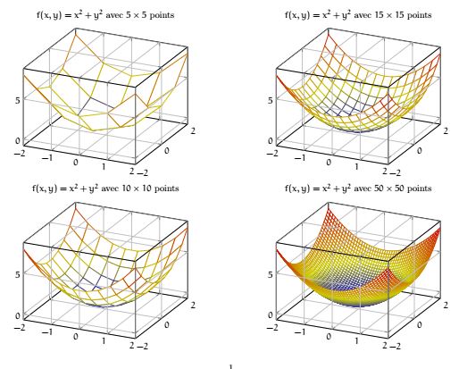
Avec les fonctions à deux variables cela est plus compliqué. Il faut réaliser le graphique en trois dimensions du graphe \( (x, y, f(x, y))\) . Sans un ordinateur cela semble difficile.
On prend différentes valeurs de \( x\) et \( y\) et on relie les points. Plus on prend de valeur plus la représentation se raffine. Il est parfois utile d'ajouter un dégradé de couleur.
%
La représentation sous différent angle de vue permet aussi de mieux appréhender la fonction.
%

Lignes de niveau et fonctions partielles
Définition
Soient \( E\subseteq \R^2\) , \( f:E\rightarrow\R\) une fonction à deux variables et \( h\in R\) . La ligne de niveau \( h\) de \( f\) est l'ensemble
\[L_h=\left\{(x, y)\in E\Big| f(x, y) = h\right\}\]
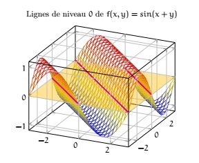
Géométriquement une ligne de niveau correspond à l'intersection de la courbe de \( f\) et du plan \( z=h\) .
Prenons par exemple la fonction définie sur \( \R^2\) : \( f(x, y)=sin(x+y)\) alors la ligne de niveau \( 0\) est l'ensemble des droite \( y=-x+k\pi\) pour \( k\in \Z\) .
%
Définition
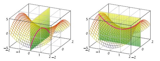
Soient \( E\subseteq \R^2\) , \( f:E\rightarrow\R\) une fonction à deux variables et \( (a, b)\in E\) . Les fonctions partielles de \( f\) en \( (a, b)\) sont définies par
\[f_{|y=b}(x)=f(x, b)\qquad f_{|x=a}(y)=f(a, y)\]
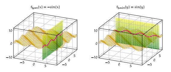
Géométriquement les fonctions partielle correspondent à l'intersection du graphe de \( f\) avec les plans \( x=a\) ou \( y=b\) .
Reprenons l'exemple de la fonction \( f(x, y)=sin(x+y)\) . Alors
\[f_{|y=\pi}(x)=-sin(x)\qquad f_{|x=2\pi}(y)=sin(y)\]
%
Dérivées partielles et gradient
L'idée est d'imiter ce que nous savons faire avec les fonctions à une variable et d'obtenir un équivalent de l'outil qu'est la dérivée.
Sauf qu'il y a un problème avec la définition de dérivé. Avec une variable le nombre dérivé d'une fonction \( f\) en un point \( a\) est défini par la limite \( \lim{x\rightarrow a}\dfrac{f(x)-f(a)}{x-a}\) . Avec une variable, la notion de limite est assez claire, soit on se rapproche de \( a\) par la gauche, ce qui est noté \( \lim{x\rightarrow a^-}\) , soit par la droite, noté \( \lim{x\rightarrow a^+}\) . En effet, sur
une ligne, on peut moralement se rapprocher d'un nombre soit par la gauche soit par la droite.
Mais lorsque nous sommes avec deux variables, quel sens donner à la notion de limite ? Comment se rapprocher d'un point. Il y a plein de manière différente de se rapproche de \( (a, b)\) : en spirale, en ligne droite, de manière exponentielle ou logarithmique, comme une parabole etc... Est-ce qu'il existe une
meilleure manière de se rapprocher d'un point ou est-ce qu'il existe un
moyen universelle ?
La réponse à cette question est OUI. Mais dans le cadre de ce cours nous n'allons pas introduire cette notion qui nécessite de définir une distance et de parler de développement limité. Une autre manière d'introduire la dérivée avec plusieurs variables est de se servir des fonctions partielles et de les dériver.
Définition
Soient \( E\subseteq \R^2\) , \( f:E\rightarrow\R\) une fonction à deux variables et \( (a, b)\in E\) .
- \( \bullet\)
- La dérivé partielle de \( f\) par rapport à \( x\) en \( (a, b)\) est la dérivé de la fonction partielle \( f_{|y=b}(x)\) en \( x=a\) . On la note \( \dfrac{\partial f}{\partial x} (a, b)\) . Par définition c'est
\[\dfrac{\partial f}{\partial x} (a, b)=\lim{x\rightarrow a}\dfrac{f(x, b)-f(a, b)}{x-a}\]
- \( \bullet\)
- La dérivé partielle de \( f\) par rapport à \( y\) en \( (a, b)\) est la dérivé de la fonction partielle \( f_{|x=a}(y)\) en \( y=b\) . On la note \( \dfrac{\partial f}{\partial y} (a, b)\) . Par définition c'est
\[\dfrac{\partial f}{\partial y} (a, b)=\lim{y\rightarrow b}\dfrac{f(a, y)-f(a, b)}{y-b}\]
On définit, comme pour les fonction à une variables, les fonctions dérivées partielles en \( (a, b)\) .
En d'autres termes, la dérivée partielle \( \dfrac{\partial f}{\partial x}\) revient à "
oublier" que \( y\) est une variable dans l'expression de \( f(x, y)\) et de ne dériver qu'en considérant \( x\) comme variable et \( y\) comme constante.
En particulier, toutes les opérations classiques sur les dérivées s'appliquent.
Prenons par exemple la fonction \( f(x, y)=\dfrac{x}{x^2+y^2}\) définie sur \( \R^2-\{(0, 0)\}\) . Alors
En utilisant la dérivé de \( \dfrac{u}{v}\) qui est \( \dfrac{u'v-v'u}{v^2}\) :
\begin{eqnarray*}
\dfrac{\partial f}{\partial x}
&=&\dfrac{(1)\times (x^2+y^2)-(x)(2x)}{(x^2+y^2)}\\
&=&\dfrac{y^2-x^2}{(x^2+y^2)}
\end{eqnarray*}
En utilisant la dérivé de \( \dfrac{1}{u}\) qui est \( -\dfrac{u'}{u^2}\) , le \( x\) au numérateur étant considéré comme une constante :
\begin{eqnarray*}
\dfrac{\partial f}{\partial y}
&=&-\dfrac{x\times 2y}{(x^2+y^2)}\\
&=&-\dfrac{2xy}{(x^2+y^2)}
\end{eqnarray*}
Avec une seule variable le nombre dérivée représentait la vitesse, précisément le vecteur vitesse (c'est la tangente).
Avec deux variables, c'est la même chose. On parle du gradient.
Définition
Soient \( E\subseteq \R^2\) , \( f:E\rightarrow\R\) une fonction à deux variables et \( (a, b)\in E\) . Le gradient de \( f\) en \( (a, b)\) est le vecteur
\[\overrightarrow{Grad}_{(a, b)}(f)=\begin{pmatrix}
\dfrac{\partial f}{\partial x}(a, b)\\
\dfrac{\partial f}{\partial y}(a, b)
\end{pmatrix}
\]
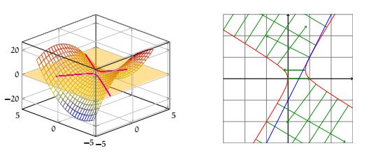
Considérons la fonction \( f(x, y) = -x^2-xy+x+y^2\) . Le gradient est \( \overrightarrow{Grad}_{(a, b)}(f)=\begin{pmatrix}
-2a-b+1\\
-a+2b
\end{pmatrix}
\) représenté en vert ci dessous.
%
Proposition
Le gradient d'une fonction en \( (a, b)\) est orthogonale à la ligne de niveau \( f(a, b)\) .
Démonstration
Admise
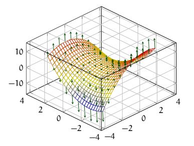
Reprenons la fonction précédente. Considérons le point \( (a, b)=(1, 1)\) . Le gradient est \( \overrightarrow{Grad}_{(1, 1)}(f)=\begin{pmatrix}
-2\\
1
\end{pmatrix}
\)
En dessin cela donne (en rouge la ligne de niveau \( f(1,1)=0\) ) en verts les gradients.
%
Corollaire
Soient \( E\subseteq \R^2\) , \( f:E\rightarrow\R\) une fonction à deux variables et \( (a, b)\in E\) tel que \( \overrightarrow{Grad}_{(a, b)}(f)\) existe et n'est pas le vecteur nul. Alors la droite tangente à la ligne de niveau \( f(a,b)\) a pour équation :
\[\dfrac{\partial f}{\partial x}(a, b)(x-a)+\dfrac{\partial f}{\partial y}(a, b)(y-b)=0\]
Démonstration
Soit \( A=(a, b)\) . Notons \( M=(x, y)\) un point de cette droite. Comme \( \overrightarrow{AM}\) est orthogonal à \( \overrightarrow{Grad}_{(a, b)}(f)\) (d'après la proposition précédente) on a \( \overrightarrow{Grad}_{(a, b)}(f)\cdot\overrightarrow{AM}=0\) ce qui traduit l'équation du corollaire.
Par exemple l'équation de la tangente en \( (1, 1)\) de la ligne de niveau \( 0\) de la fonction \( f(x, y) = -x^2-xy+x+y^2\) est \( -2(x-1)+1(y-1)=0\) soit la droite \( y=2x-1\) (en bleue sur le graphique précédent).
Que se passe-t-il si le gradient est nul ?
Extrema globaux et locaux
Définition
Soient \( E\subseteq \R^2\) , \( f:E\rightarrow\R\) une fonction à deux variables et \( (a, b)\in E\) .
- \( \bullet\)
- On dira que \( (a, b)\) est un maximum (resp. minimum) global si pour tout \( (x, y)\in E\) , \( f(x, y)\leqslant f(a, b)\) (resp. \( f(x, y)\geqslant f(a, b)\) ).
- \( \bullet\)
- On dira que \( (a, b)\) est un maximum (resp. minimum) global si pour tout \( (x, y)\in D\) , \( f(x, y)\leqslant f(a, b)\) (resp. \( f(x, y)\geqslant f(a, b)\) ).
Où \( D\subset E\) est un (petit) disque autour de \( (a, b)\) .
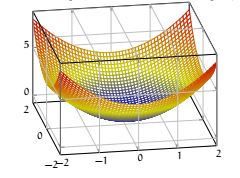
Par exemple, il est facile d'observer que \( (0, 0)\) est un minimum global de \( f(x, y)=x^2+y^2\) .
%
Définition
Soient \( E\subseteq \R^2\) , \( f:E\rightarrow\R\) une fonction à deux variables et \( (a, b)\in E\) .
On dira que \( (a, b)\) est un point critique si \( \overrightarrow{Grad}_{(a, b)}(f)=\overrightarrow{0}\) .
Reprenons l'exemple de la fonction \( f(x, y) = -x^2-xy+x+y^2\) et dont le gradient est \( \overrightarrow{Grad}_{(a, b)}(f)=\begin{pmatrix}
-2a-b+1\\
-a+2b
\end{pmatrix}
\) . Trouver les points critiques revient donc à résoudre le système
\[
\left\{
\begin{array}{rcl}
-2a-b+1=0\\
-a+2b=0
\end{array}
\right.
\]
Il est facile de voir que ce système admet une unique solution \( (a, b)=\left(\dfrac{1}{5}, \dfrac{2}{5}\right)\) . En conclusion, l'unique point critique de cette fonction est \( \left(\dfrac{1}{5}, \dfrac{2}{5}\right)\) .
Théorème [Fermat]
Soient \( E\subseteq \R^2\) , \( f:E\rightarrow\R\) une fonction à deux variables et \( (a, b)\in E\) .
Si \( (a, b)\) est un extrema local alors c'est un point critique.
Démonstration
Admise
En conclusion, pour déterminer un extremum, il suffit de déterminer les points critiques d'une fonction. Mais comment savoir si c'est un maximum ou un minimum. Réalisons quelques exemple à une variables.
Considérons la fonction \( f(x)=x^2\) . Sa dérivé est \( f'(x)=2x\) qui s'annule trivialement en \( x=0\) . Ainsi \( 0\) est un point critique. Nous savons, en regardant le graphique que c'est un minimum. Regardons la dérivé seconde : \( f''(x)=2\) ... c'est positif en \( x=0\) .
Considérons la fonction \( f(x)=-x^2\) . Sa dérivé est \( f'(x)=-2x\) qui s'annule trivialement en \( x=0\) . Ainsi \( 0\) est un point critique. Nous savons, en regardant le graphique que c'est un maximum. Regardons la dérivé seconde : \( f''(x)=-2\) ... c'est négatif en \( x=0\) .
Considérons la fonction \( f(x)=x^3\) . Sa dérivé est \( f'(x)=3x^2\) qui s'annule trivialement en \( x=0\) . Ainsi \( 0\) est un point critique. Regardons la dérivé seconde : \( f''(x)=6x\) ... nul en \( x=0\) .
Vous l'aurez compris, c'est en regardant du coté de la dérivé seconde que nous aurons une réponse.
La hessienne
Il nous faut définir la
dérivée seconde. Nous avons les dérivés premiers \( \dfrac{\partial f}{\partial x}\) et \( \dfrac{\partial f}{\partial y}\) . Ce sont des fonctions à deux variables que nous pouvons encore dériver par rapport à la première ou la seconde variable.
Définition
Soient \( E\subseteq \R^2\) , \( f:E\rightarrow\R\) une fonction à deux variables. Si elles existent, on note
\[\dfrac{\partial}{\partial x}\left(\dfrac{\partial f}{\partial x}\right) = \dfrac{\partial^2 f}{\partial x^2}\]
\[\dfrac{\partial}{\partial x}\left(\dfrac{\partial f}{\partial y}\right) = \dfrac{\partial^2 f}{\partial x\partial y}\]
\[\dfrac{\partial}{\partial y}\left(\dfrac{\partial f}{\partial x}\right) = \dfrac{\partial^2 f}{\partial y\partial x}\]
\[\dfrac{\partial}{\partial y}\left(\dfrac{\partial f}{\partial y}\right) = \dfrac{\partial^2 f}{\partial y^2}\]
Prenons par exemple \( f(x, y)=-x^2-xy+x+y^2\) alors
\[\dfrac{\partial^2 f}{\partial x^2}=\dfrac{\partial}{\partial x}(-2x-y+1)=-2\]
\[\dfrac{\partial^2 f}{\partial x\partial y}=\dfrac{\partial}{\partial x}(-x+2y)=-1\]
\[\dfrac{\partial^2 f}{\partial y\partial x}=\dfrac{\partial}{\partial y}(-2x-y+1)=-1\]
\[\dfrac{\partial^2 f}{\partial y^2}=\dfrac{\partial}{\partial y}(-x+2y)=2\]
On observe que \( \dfrac{\partial^2 f}{\partial x\partial y}=\dfrac{\partial^2 f}{\partial y\partial x}\) . C'est toujours vrai.
Théorème [Lemme de Schwartz]
\[\dfrac{\partial^2 f}{\partial x\partial y}=\dfrac{\partial^2 f}{\partial y\partial x}\]
Démonstration
\begin{eqnarray*}
\dfrac{\partial^2 f}{\partial x\partial y}(a, b)
&=& \lim{x\rightarrow a}\dfrac{\dfrac{\partial f}{\partial y} (x, b)-\dfrac{\partial f}{\partial y} (a, b)}{x-a}\\
&=& \lim{x\rightarrow a}\dfrac{\lim{y\rightarrow b}\dfrac{f(x, y)-f(x, b)}{y-b} -\lim{y\rightarrow b}\dfrac{f(a, y)-f(a, b)}{y-b} }{x-a}\\
&=& \lim{x\rightarrow a}\dfrac{\lim{y\rightarrow b}\left[\dfrac{f(x, y)-f(x, b)}{y-b} -\dfrac{f(a, y)-f(a, b)}{y-b} \right]}{x-a}\\
&=& \lim{x\rightarrow a}\dfrac{\lim{y\rightarrow b}\left[\dfrac{(f(x, y)-f(x, b))-(f(a, y)-f(a, b))}{y-b}\right]}{x-a}\\
&=& \lim{y\rightarrow b}\lim{x\rightarrow a}\dfrac{\left[\dfrac{(f(x, y)-f(x, b))-(f(a, y)-f(a, b))}{y-b}\right]}{x-a}\\
&=& \lim{y\rightarrow b}\lim{x\rightarrow a}\dfrac{\left[\dfrac{(f(x, y)-f(x, b))-(f(a, y)-f(a, b))}{x-a}\right]}{y-b}\\
&=& \lim{y\rightarrow b}\lim{x\rightarrow a}\dfrac{\left[\dfrac{(f(x, y)-f(a, y))-(f(x, b)-f(a, b))}{x-a}\right]}{y-b}\\
&=& \lim{y\rightarrow b}\lim{x\rightarrow a}\dfrac{\left[\dfrac{f(x, y)-f(a, y)}{x-a} - \dfrac{f(x, b)-f(a, b)}{x-a}\right]}{y-b}\\
&=& \lim{y\rightarrow b}\dfrac{\lim{x\rightarrow a}\left[\dfrac{f(x, y)-f(a, y)}{x-a} - \dfrac{f(x, b)-f(a, b)}{x-a}\right]}{y-b}\\
&=& \lim{y\rightarrow b}\dfrac{\lim{x\rightarrow a}\dfrac{f(x, y)-f(a, y)}{x-a} - \lim{x\rightarrow a}\dfrac{f(x, b)-f(a, b)}{x-a}}{y-b}\\
&=& \lim{y\rightarrow b}\dfrac{\dfrac{\partial f}{\partial x}(a, y) - \dfrac{\partial f}{\partial x}(a, b)}{y-b}\\
&=& \dfrac{\partial f^2}{\partial y \partial x}(a, b)
\end{eqnarray*}
Définition
Soient \( E\subseteq \R^2\) , \( f:E\rightarrow\R\) une fonction à deux variables et \( (a, b)\in E\) .
La matrice hessienne de \( f\) est la matrice
\[
H_{(a, b)}(f)
=\begin{pmatrix}
\dfrac{\partial^2 f}{\partial x^2}(a, b) & \dfrac{\partial^2 f}{\partial x\partial y} (a, b)\\
\dfrac{\partial^2 f}{\partial y\partial x}(a, b)&\dfrac{\partial^2 f}{\partial y^2}(a, b)
\end{pmatrix}
\]
Par exemple la hessienne de \( f(x, y)=-x^2-xy+x+y^2\) (en tout point) est \( \begin{pmatrix}
-2&-1\\
-1&2
\end{pmatrix}\)
Théorème
Soient \( E\subseteq \R^2\) , \( f:E\rightarrow\R\) une fonction à deux variables, \( (a, b)\) un point critique et \( H\) sa matrice hessienne.
- Si \( \det(H){>}0\)
- et
- si \( tr(H){>}0\)
- alors \( (a, b)\) est un minimum local.
- si \( tr(H){<}0\)
- alors \( (a, b)\) est un maximum local.
- Si \( \det(H){<}0\)
- alors \( (a, b)\) est un point selle.
- Si \( \det(H)=0\)
- alors on ne peut pas conclure. On dit que \( (a,b)\) est un point critique dégénéré.
Démonstration
Admise.
Rappelons que pour une matrice carré en dimension \( 2\) , le déterminant
\( \det\begin{pmatrix}
a&b\\
c&d
\end{pmatrix}=ad-bc
\) et la trace
\( tr\begin{pmatrix}
a&b\\
c&d
\end{pmatrix}=a+d\)
§
On peut démontrer que si \( \det(H){>}0\) alors la trace est nécessairement non nulle de sorte que nous n'avons pas oublié de traiter un cas dans le théorème précédent.
Par exemple nous avions trouver que le point critique de la fonction \( f(x, y) = -x^2-xy+x+y^2\) est \( \left(\dfrac{1}{5}, \dfrac{2}{5}\right)\) .
La hessienne est \( \begin{pmatrix}
-2&-1\\
-1&2
\end{pmatrix}\) . Son déterminant vaut \( -5\) . Le point \( \left(\dfrac{1}{5}, \dfrac{2}{5}\right)\) est un point selle.
§
Si la notion de minimum et de maximum est assez claire, celle de
point selle est un peu plus exotique. C'est un point qui n'est ni un maximum ni un minimum mais aussi les deux en même temps.
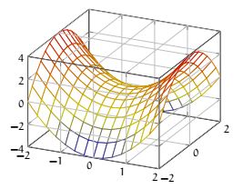
Regardons la fonction définie sur \( \R^2\) , \( f(x, y)=x^2-y^2\) .
On vérifie que
\( \overrightarrow{Grad} f=\begin{pmatrix}
2x\\
-2y
\end{pmatrix}
\) et on observe trivialement que le seul point critique est \( (0, 0)\) . On vérifie également que la hessienne
\(
\begin{pmatrix}
2&0\\
0&-2
\end{pmatrix}
\) . D'après le théorème précédent le point critique est un point selle : selon une direction la fonction est croissante et selon une autre elle est décroissante... comme une selle de cheval, d'où le nom.
%
%
Et plus de deux variables ?
Si on dispose d'une fonction de plus de deux variables, les concepts sont les mêmes !
Cependant l'étude du déterminant et de la trace de la hessienne ne suffit pas pour déterminer la nature du point critique.
Le théorème spectrale devrait être un outil puissant, mais hors de propos dans ce cours.
Pour étudier la fonction définie sur \( \R^3\) par \( f(x, y, z)=x^2+yz+z\) , on commence par chercher les points critique par le calcul du gradient.
On trouve aisément que \( \overrightarrow{Grad} (f)=
\begin{pmatrix}
2x\\
z\\
y+1
\end{pmatrix}
\)
qui s'annule en \( (x, y, z)=(0, -1, 0)\) . On détermine sa hessienne tout aussi aisément :
\( H=
\begin{pmatrix}
2&0&0\\
0&0&1\\
0&1&0
\end{pmatrix}
\) . On a \( \det(H)=-2{<}0\) et \( tr(H)=2{>}0\) et le point \( (0, -1, 0)\) est une sorte de point selle : il existe deux directions différentes selon lesquelles la fonction est croissante pour l'une et décroissante pour l'autre.


