Il nous faut définir la
dérivée seconde. Nous avons les dérivés premiers \( \dfrac{\partial f}{\partial x}\) et \( \dfrac{\partial f}{\partial y}\) . Ce sont des fonctions à deux variables que nous pouvons encore dériver par rapport à la première ou la seconde variable.
Définition
Soient \( E\subseteq \R^2\) , \( f:E\rightarrow\R\) une fonction à deux variables. Si elles existent, on note
\[\dfrac{\partial}{\partial x}\left(\dfrac{\partial f}{\partial x}\right) = \dfrac{\partial^2 f}{\partial x^2}\]
\[\dfrac{\partial}{\partial x}\left(\dfrac{\partial f}{\partial y}\right) = \dfrac{\partial^2 f}{\partial x\partial y}\]
\[\dfrac{\partial}{\partial y}\left(\dfrac{\partial f}{\partial x}\right) = \dfrac{\partial^2 f}{\partial y\partial x}\]
\[\dfrac{\partial}{\partial y}\left(\dfrac{\partial f}{\partial y}\right) = \dfrac{\partial^2 f}{\partial y^2}\]
Prenons par exemple \( f(x, y)=-x^2-xy+x+y^2\) alors
\[\dfrac{\partial^2 f}{\partial x^2}=\dfrac{\partial}{\partial x}(-2x-y+1)=-2\]
\[\dfrac{\partial^2 f}{\partial x\partial y}=\dfrac{\partial}{\partial x}(-x+2y)=-1\]
\[\dfrac{\partial^2 f}{\partial y\partial x}=\dfrac{\partial}{\partial y}(-2x-y+1)=-1\]
\[\dfrac{\partial^2 f}{\partial y^2}=\dfrac{\partial}{\partial y}(-x+2y)=2\]
On observe que \( \dfrac{\partial^2 f}{\partial x\partial y}=\dfrac{\partial^2 f}{\partial y\partial x}\) . C'est toujours vrai.
Théorème [Lemme de Schwartz]
\[\dfrac{\partial^2 f}{\partial x\partial y}=\dfrac{\partial^2 f}{\partial y\partial x}\]
Démonstration
\begin{eqnarray*}
\dfrac{\partial^2 f}{\partial x\partial y}(a, b)
&=& \lim{x\rightarrow a}\dfrac{\dfrac{\partial f}{\partial y} (x, b)-\dfrac{\partial f}{\partial y} (a, b)}{x-a}\\
&=& \lim{x\rightarrow a}\dfrac{\lim{y\rightarrow b}\dfrac{f(x, y)-f(x, b)}{y-b} -\lim{y\rightarrow b}\dfrac{f(a, y)-f(a, b)}{y-b} }{x-a}\\
&=& \lim{x\rightarrow a}\dfrac{\lim{y\rightarrow b}\left[\dfrac{f(x, y)-f(x, b)}{y-b} -\dfrac{f(a, y)-f(a, b)}{y-b} \right]}{x-a}\\
&=& \lim{x\rightarrow a}\dfrac{\lim{y\rightarrow b}\left[\dfrac{(f(x, y)-f(x, b))-(f(a, y)-f(a, b))}{y-b}\right]}{x-a}\\
&=& \lim{y\rightarrow b}\lim{x\rightarrow a}\dfrac{\left[\dfrac{(f(x, y)-f(x, b))-(f(a, y)-f(a, b))}{y-b}\right]}{x-a}\\
&=& \lim{y\rightarrow b}\lim{x\rightarrow a}\dfrac{\left[\dfrac{(f(x, y)-f(x, b))-(f(a, y)-f(a, b))}{x-a}\right]}{y-b}\\
&=& \lim{y\rightarrow b}\lim{x\rightarrow a}\dfrac{\left[\dfrac{(f(x, y)-f(a, y))-(f(x, b)-f(a, b))}{x-a}\right]}{y-b}\\
&=& \lim{y\rightarrow b}\lim{x\rightarrow a}\dfrac{\left[\dfrac{f(x, y)-f(a, y)}{x-a} - \dfrac{f(x, b)-f(a, b)}{x-a}\right]}{y-b}\\
&=& \lim{y\rightarrow b}\dfrac{\lim{x\rightarrow a}\left[\dfrac{f(x, y)-f(a, y)}{x-a} - \dfrac{f(x, b)-f(a, b)}{x-a}\right]}{y-b}\\
&=& \lim{y\rightarrow b}\dfrac{\lim{x\rightarrow a}\dfrac{f(x, y)-f(a, y)}{x-a} - \lim{x\rightarrow a}\dfrac{f(x, b)-f(a, b)}{x-a}}{y-b}\\
&=& \lim{y\rightarrow b}\dfrac{\dfrac{\partial f}{\partial x}(a, y) - \dfrac{\partial f}{\partial x}(a, b)}{y-b}\\
&=& \dfrac{\partial f^2}{\partial y \partial x}(a, b)
\end{eqnarray*}
Définition
Soient \( E\subseteq \R^2\) , \( f:E\rightarrow\R\) une fonction à deux variables et \( (a, b)\in E\) .
La matrice hessienne de \( f\) est la matrice
\[
H_{(a, b)}(f)
=\begin{pmatrix}
\dfrac{\partial^2 f}{\partial x^2}(a, b) & \dfrac{\partial^2 f}{\partial x\partial y} (a, b)\\
\dfrac{\partial^2 f}{\partial y\partial x}(a, b)&\dfrac{\partial^2 f}{\partial y^2}(a, b)
\end{pmatrix}
\]
Par exemple la hessienne de \( f(x, y)=-x^2-xy+x+y^2\) (en tout point) est \( \begin{pmatrix}
-2&-1\\
-1&2
\end{pmatrix}\)
Théorème
Soient \( E\subseteq \R^2\) , \( f:E\rightarrow\R\) une fonction à deux variables, \( (a, b)\) un point critique et \( H\) sa matrice hessienne.
- Si \( \det(H){>}0\)
- et
- si \( tr(H){>}0\)
- alors \( (a, b)\) est un minimum local.
- si \( tr(H){<}0\)
- alors \( (a, b)\) est un maximum local.
- Si \( \det(H){<}0\)
- alors \( (a, b)\) est un point selle.
- Si \( \det(H)=0\)
- alors on ne peut pas conclure. On dit que \( (a,b)\) est un point critique dégénéré.
Démonstration
Admise.
Rappelons que pour une matrice carré en dimension \( 2\) , le déterminant
\( \det\begin{pmatrix}
a&b\\
c&d
\end{pmatrix}=ad-bc
\) et la trace
\( tr\begin{pmatrix}
a&b\\
c&d
\end{pmatrix}=a+d\)
§
On peut démontrer que si \( \det(H){>}0\) alors la trace est nécessairement non nulle de sorte que nous n'avons pas oublié de traiter un cas dans le théorème précédent.
Par exemple nous avions trouver que le point critique de la fonction \( f(x, y) = -x^2-xy+x+y^2\) est \( \left(\dfrac{1}{5}, \dfrac{2}{5}\right)\) .
La hessienne est \( \begin{pmatrix}
-2&-1\\
-1&2
\end{pmatrix}\) . Son déterminant vaut \( -5\) . Le point \( \left(\dfrac{1}{5}, \dfrac{2}{5}\right)\) est un point selle.
§
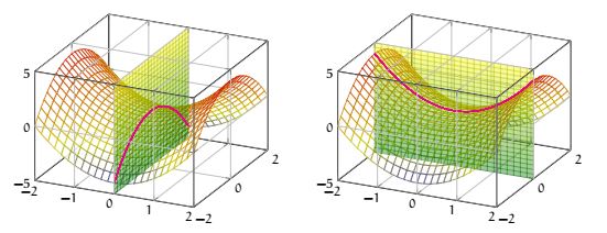
Si la notion de minimum et de maximum est assez claire, celle de
point selle est un peu plus exotique. C'est un point qui n'est ni un maximum ni un minimum mais aussi les deux en même temps.
Regardons la fonction définie sur \( \R^2\) , \( f(x, y)=x^2-y^2\) .
On vérifie que
\( \overrightarrow{Grad} f=\begin{pmatrix}
2x\\
-2y
\end{pmatrix}
\) et on observe trivialement que le seul point critique est \( (0, 0)\) . On vérifie également que la hessienne
\(
\begin{pmatrix}
2&0\\
0&-2
\end{pmatrix}
\) . D'après le théorème précédent le point critique est un point selle : selon une direction la fonction est croissante et selon une autre elle est décroissante... comme une selle de cheval, d'où le nom.
%

%